Welcome👋,

In this article, we are going to build our own KNN algorithm from scratch and apply it to 23 different feature data set using Numpy and Pandas libraries.

First, let us get some idea about the KNN or K Nearest Neighbour algorithm.

What is the K Nearest Neighbors algorithm?

K Nearest Neighbors is one of the simplest predictive algorithms out there in the supervised machine learning category.

The algorithm works based on two criteria: —

• The number of neighbours to include in the cluster.
• The distance of the neighbours from the test data point.

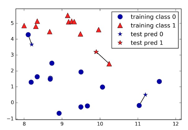
Fig: Prediction made by one nearest neighbour (book: Intro to Machine Learning with Python)

The above image showcases the number of neighbours (k = the number of neighbours) that are being considered in predicting the value for the test data point.

Now, let us start coding in our jupyter notebook.

Let's Code

Data Preprocessing

In our case, we are using the diamonds dataset having 10 features out of which 3 are categorical and the rest 7 are numerical features.

Removing Outliers

We can use the boxplot() function to produce boxplots and check if there are any outliers present in the dataset.

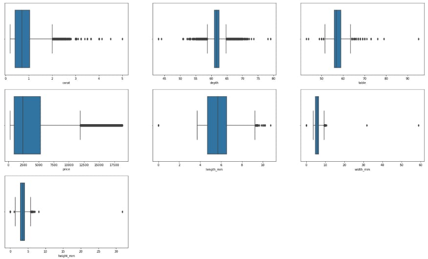
We can see that there are some outliers in the dataset.

So we remove these outliers using the IQR method (or choose any method of your choice).

# IQR
def remove_outlier_IQR(df, field_name):
    iqr = 1.5 * (np.percentile(df[field_name], 75) -
                 np.percentile(df[field_name], 25))
    df.drop(df[df[field_name] > (
        iqr + np.percentile(df[field_name], 75))].index, inplace=True)
    df.drop(df[df[field_name] < (np.percentile(
        df[field_name], 25) - iqr)].index, inplace=True)
return df

Printing the shape of the data frame before and after outlier removal using IQR.

print('Shape of df before IQR:',df.shape)

df2 = remove_outlier_IQR(df, 'carat')
df2 = remove_outlier_IQR(df2, 'depth')
df2 = remove_outlier_IQR(df2, 'price')
df2 = remove_outlier_IQR(df2, 'table')
df2 = remove_outlier_IQR(df2, 'height_mm')
df2 = remove_outlier_IQR(df2, 'length_mm')
df_final = remove_outlier_IQR(df2, 'width_mm')
print('The Shape of df after IQR:',df_final.shape)

The shape of df before IQR: (53940, 10)

The shape of df after IQR: (46518, 10)

Again, after removing the outliers, we check the dataset using a boxplot for better visual confirmation.

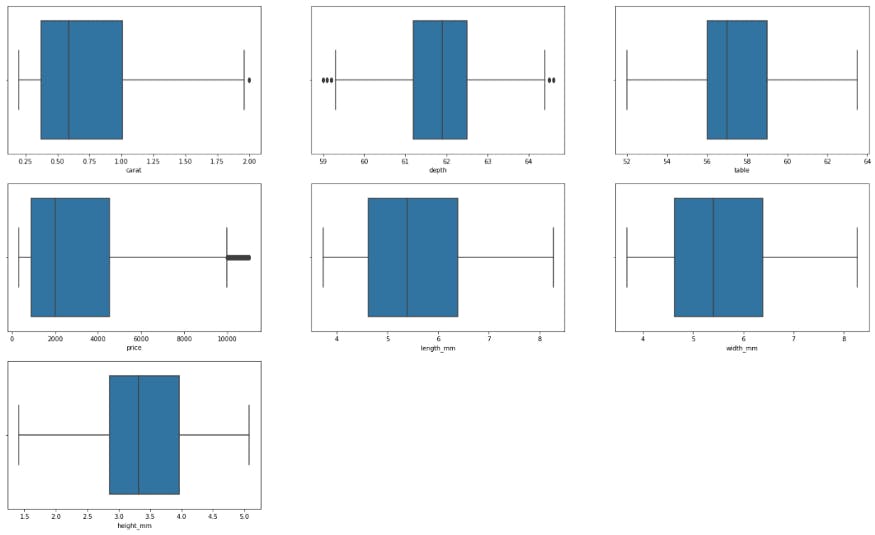
Boxplots after IQR method

Encoding the Categorical variables

There are 3 categorical features in the dataset. Let us print and see the unique values of each feature.

print('Unique values of cat features:\n')
print('color:', cat_df.color.unique())
print('cut_quality:', cat_df.cut_quality.unique())
print('clarity:', cat_df.clarity.unique())

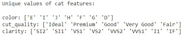
These are the unique values of the categorical features.

So, for encoding these features, we use LabelEncoder and Dummy variables (or you can also use OneHotEncoder)

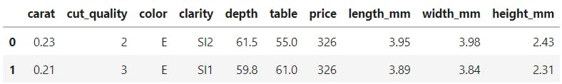
We can use LabelEncoder() for converting the cut_quality to numerical values like 0, 1, 2, ….. because cut_quality has ordinal data.

# Label encoding using the LabelEncoder function from sklearn
from sklearn.preprocessing import LabelEncoder
label_encoder = LabelEncoder()

df_final['cut_quality'] = label_encoder.fit_transform(df_final['cut_quality'])
df_final.head(2)

Then we use the get_dummies() function of the pandas library to get the dummy variables for the categories colour and clarity.

# using dummy variables for the remaing categories
df_final = pd.get_dummies(df_final,columns=['color','clarity'])
df_final.head()

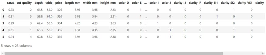
df_final.shape
--> (46518, 23)

Splitting data for training and testing

We split the data for training and testing using the train_test_split() method from the sklearn library. The test_size is kept to be equal to 25% of the original dataset.

data = df_final.copy()
# Using sklearn for scaling and splitting
from sklearn.preprocessing import StandardScaler
from sklearn.model_selection import train_test_split

X = data.drop(columns=['price'])
y = data['price']

# Scaling the data
scaler = StandardScaler()
scaled_df = scaler.fit_transform(X)

X_train, X_test, y_train, y_test = train_test_split(
    scaled_df, y, test_size=0.25)
print("X train shape: {} and y train shape: {}".format(
    X_train.shape, y_train.shape))
print("X test shape: {} and y test shape: {}".format(X_test.shape, y_test.shape))

KNN from sklearn library Vs KNN built from scratch

Sklearn KNN model

First we use KNN regressor model from sklearn.

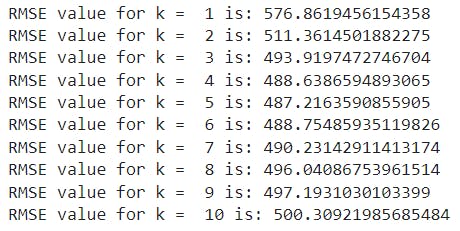
For choosing the optimal k value, we iterate using for loop putting the k value from 1 to 10.

In our case, the optimal k value obtained is 5. So using this k = 5 we train the model and make predictions and print those predicted values.

# Finding the optimal k value
from sklearn import neighbors
from sklearn.metrics import mean_squared_error
from math import sqrt
import matplotlib.pyplot as plt
rmse_val = []  
for K in range(10):
    K = K+1
    model = neighbors.KNeighborsRegressor(n_neighbors=K)

    model.fit(X_train, y_train)  
    pred = model.predict(X_test)  
    error = sqrt(mean_squared_error(y_test, pred))  
    rmse_val.append(error)  
    print('RMSE value for k = ', K, 'is:', error)

# Using the optimal k value.
from sklearn import neighbors

model = neighbors.KNeighborsRegressor(n_neighbors=5)

model.fit(X_train, y_train)  # fit the model
pred = model.predict(X_test)
pred

Now, let's move on to our own KNN model from sklearn using NumPy and pandas.

KNN model from scratch

We convert the train and test data into NumPy arrays.

Then we combine the X_train and y_train into a matrix.

The matrix will contain the 22 columns of the X_train data and 1 column of the y_train at the end (i.e the last column).

train = np.array(X_train)
test = np.array(X_test)
y_train = np.array(y_train)
# reshaping the array from columns to rows
y_train = y_train.reshape(-1, 1)
# combining the training dataset and the y_train into a matrix
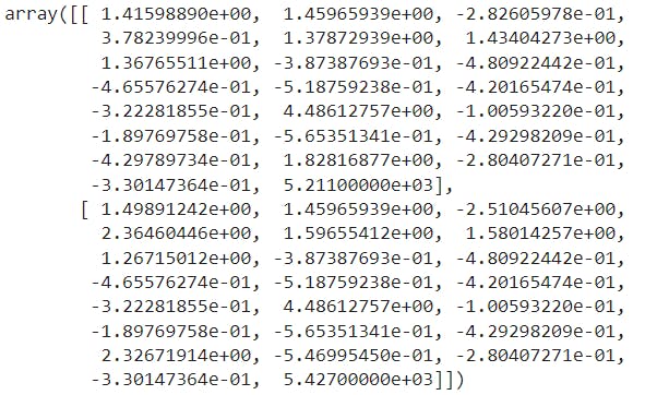
train_df = np.hstack([train, y_train])
train_df[0:2]

Now, for each row (data point) of the test dataset, we find the euclidian distance between every point of the train data and the test data point.

We use for loop for iterating through every point on the test dataset to find the distances and stacking them into the training dataset train_df respectively.

Steps:

1. We find the distances between one test point and every point of the train data set.
2. We reshape the distances using reshape(-1,1) to convert this into an array of 1 column and the 11630 rows.
3. Then using np.hstack() we stack this distance array into the train_df dataset.
4. Now we sort this matrix from smallest to largest based on the distance column.
5. We then take the y_train values from the first 5 rows and take their mean to obtain the prediction value.
6. Repeat the above steps for every test point and predict the values respectively and store these values in an array.

preds = []
for i in range(len(test)):
    distances = np.sqrt(np.sum((train - test[i])**2, axis = 1))
    distances = distances.reshape(-1,1)
    matrix = np.hstack([train_df, distances])
    sorted_matrix = matrix[matrix[:,-1].argsort()]
    neighbours = [sorted_matrix[i][-2] for i in range(5)]
    pred_value = np.mean(neighbours)
    preds.append(pred_value)
knn_scratch_pred = np.array(preds)
knn_scratch_pred

Comparing Sklearn and Our KNN model

For comparing the prediction values obtained from sklearn and our knn_method, we produce a pandas data frame pred_df as shown in the code below.

sklearn_pred = pred.reshape(-1,1)
my_knn_pred = knn_scratch_pred.reshape(-1,1)
predicted_values = np.hstack([sklearn_pred,my_knn_pred])
pred_df = pd.DataFrame(predicted_values,columns=['sklearn_preds','my_knn_preds'])
pred_df

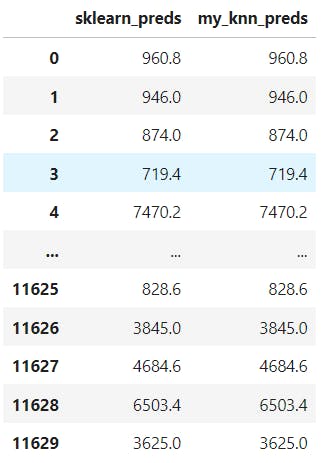
We can see that the predicted values of our knn_algorithm are exactly similar to those obtained using the sklearn library. This shows that our intuition and method is correct and very accurate.

For the full code file and the dataset, visit Github.

---

🌎Explore, 🎓Learn, 👷‍♂️Build. Happy Coding💛